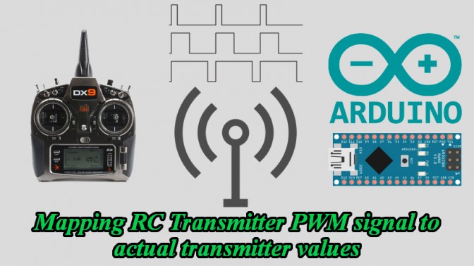
Introduction

If you ever need to use an RC Transmitter & receiver for a personal project, an easy way to retrieve the signal is to connect the receiver to a micro-controller.

However, decoding the signal to get actual transmitter values is not as easy as it sounds. You need to know the correct encoding and searching on the internet about the subject gives erratic results.

Here is the full article that explains how to correctly map an RC Transmitter PWM signal to actual transmitter values.

How does it works?

The receiver signal is encoded with a Pulse Width Modulation. In other way, the transfer of the signal is analog and not digital. This means there is no direct method to read the signal. To accurately read the signal, you need to know the given length of the pulse for each unique transmitter values.

Using benchmark data, I managed to find approximation functions that works for most transmitter values. Multiple benchmark data is available for multiple combination of transmitter and receiver.

What is expected

If you search on the internet, you will find information regarding servos which typically uses the same “kind” of PWM signal. However, as you will see in the next section, the minimum and maximum values for a servo does not match their counterpart on a RC transmitter.

Theoretical values

Most information sources about servo control states that generally the minimum pulse will be about 1 ms wide and the maximum pulse will be 2 ms wide.

The following table shows the theoretical pulse length for each transmitter values:

Expected Transmitter Pulses
Length (µS)	Value
1000	-100%
1500	0%
2000	100%

Extrapolation

Knowing that a pulse delta time of 1000 µS (from 1000 µS to 2000 µS) is required to identify 200 different steps (from -100% to +100%), it is then safe to assume that each step is 5 µS. With this calculation, the theoretical pulse length of other values should be identified as follows:

Extrapolated Transmitter Pulses
Length (µS)	Value
750	-150%
875	-125%
1125	-75%
1250	-50%
1375	-25%
1625	25%
1750	50%
1875	75%
2125	125%
2250	150%

WRONG!

Theoretical values is never as good as real world observations.

Capture methodology

For the data capture, I used an Arduino Nano V3 micro-controller. With the help of multiple libraries, I created a program to capture each pulse length of critical target point for a given amount of time. Since the length of each pulse is not perfectly constant, I extracted the average pulse length. Matching different points, I calculated multiple trend line formulas in polynomial format. I then calculate each formula performance against all other points. Finally, I identify the best formula to be used in real projects.

Note that all raw data capture are available for download as Excel files (*.xlsx) in sections below.

Required Libraries

PinChangeInt

This library allows the arduino to attach interrupts on multiple pins.

eRCaGuy_Timer2_Counter

This library configures the arduino’s timer2 to 0.5µs precision. It is used for a “micros()” function replacement and allows times calculations that are far more precise (8 times!) than the default’s 4µs resolution.

PWM capture code

Here is the final arduino code that allowed raw data capture to extract average pulse length for each critical target point:

#include <PinChangeInt.h>
#include <eRCaGuy_Timer2_Counter.h>

//project's contants
#define RECEIVER_AUX1_IN_PIN 2 // we could choose any pin
#define BUFFER_SIZE 250

//project's switches
#define ENABLE_SERIAL_OUTPUT

//DECLARE_RECEIVER_SIGNAL(receiver_aux1_handler);
volatile unsigned long risingTime; //time in micros() on last pin rise
volatile unsigned long fallingTime; //time in micros() on last pin fall
volatile unsigned long pwmValue; //PWM value expected from 1000 us to 2000 us
         unsigned long prevPwmValue; //previous value of pwmValue

unsigned long readingsBuffer[BUFFER_SIZE];
unsigned long numReadings = 0;

unsigned long getPwmValue() {
  uint8_t pushedSREG = SREG;            // save interrupt flag
  cli();                                // disable interrupts
  unsigned long pwmCopy = pwmValue;    // access the shared data
  SREG = pushedSREG;                    // restore the interrupt flag

  return pwmCopy;
}

bool hasChanged() {
  unsigned long currentValue = getPwmValue();
  bool changed = (currentValue != prevPwmValue);
  prevPwmValue = currentValue;
  return changed;
}

void onPinChanged() {
  if(PCintPort::pinState == HIGH)
  {
    //this is a rising edge
    //record time
    risingTime = timer2.get_count(); //count units of 0.5us each
  }
  else
  {
    //this is a falling edge
    //read elapsed time since RISING
    fallingTime = timer2.get_count(); //count units of 0.5us each;
    pwmValue = (fallingTime - risingTime)/2; //to a precision of 1us
  }
}

void setup() {
  risingTime = 0;
  fallingTime = 0;
  pwmValue = 0;

  //setup interrupts
  pinMode(RECEIVER_AUX1_IN_PIN, INPUT);
  digitalWrite(RECEIVER_AUX1_IN_PIN, HIGH); //use the internal pullup resistor
  
  //prepare first interruption on pin CHANGE
  PCintPort::attachInterrupt(RECEIVER_AUX1_IN_PIN, &onPinChanged, CHANGE);
  
  //configure Timer2
  timer2.setup(); //this MUST be done before the other Timer2_Counter functions work; Note: since this messes up PWM outputs on pins 3 & 11, as well as 
                  //interferes with the tone() library (http://arduino.cc/en/reference/tone), you can always revert Timer2 back to normal by calling 
                  //timer2.unsetup()
  
  #ifdef ENABLE_SERIAL_OUTPUT
    Serial.begin(115200);
    Serial.println("ready");
  #endif
}

void loop() {

  //detect when the receiver AUX1 value has changed
  if (hasChanged())
  {
    unsigned long pwmValue = getPwmValue();

    //add value to reading buffer
    readingsBuffer[numReadings] = pwmValue;
    numReadings++;

    if (numReadings == BUFFER_SIZE)
    {
      //flush
      #ifdef ENABLE_SERIAL_OUTPUT
        char pwnStr[10];
        unsigned long sum = 0;
        for(unsigned long i=0; i<BUFFER_SIZE; i++)
        {
          pwmValue = readingsBuffer[i];
          sum += pwmValue;
          sprintf(pwnStr, "%04d", pwmValue);
          Serial.println(pwnStr);
        }
        double avg = sum/double(BUFFER_SIZE);
        //Serial.print("sum=");
        //Serial.println(sum);
        //Serial.print("avg=");
        //Serial.println(avg);
      #endif

      numReadings = 0;

      //ignore the next change since serial printing may have impacted the timing...
      while( !hasChanged() )
      {
      }
      
    }
  }
}

100

101

102

103

104

105

106

107

108

109

110

111

112

113

114

115

#include <PinChangeInt.h>

#include <eRCaGuy_Timer2_Counter.h>

//project's contants

#define RECEIVER_AUX1_IN_PIN 2 // we could choose any pin

#define BUFFER_SIZE 250

//project's switches

#define ENABLE_SERIAL_OUTPUT

//DECLARE_RECEIVER_SIGNAL(receiver_aux1_handler);

volatile unsigned long risingTime; //time in micros() on last pin rise

volatile unsigned long fallingTime; //time in micros() on last pin fall

volatile unsigned long pwmValue; //PWM value expected from 1000 us to 2000 us

unsigned long prevPwmValue; //previous value of pwmValue

unsigned long readingsBuffer[BUFFER_SIZE];

unsigned long numReadings = 0;

unsigned long getPwmValue() {

uint8_t pushedSREG = SREG; // save interrupt flag

cli(); // disable interrupts

unsigned long pwmCopy = pwmValue; // access the shared data

SREG = pushedSREG; // restore the interrupt flag

return pwmCopy;

}

bool hasChanged() {

unsigned long currentValue = getPwmValue();

bool changed = (currentValue != prevPwmValue);

prevPwmValue = currentValue;

return changed;

}

void onPinChanged() {

if(PCintPort::pinState == HIGH)

{

//this is a rising edge

//record time

risingTime = timer2.get_count(); //count units of 0.5us each

}

else

{

//this is a falling edge

//read elapsed time since RISING

fallingTime = timer2.get_count(); //count units of 0.5us each;

pwmValue = (fallingTime - risingTime)/2; //to a precision of 1us

}

void setup() {

risingTime = 0;

fallingTime = 0;

pwmValue = 0;

//setup interrupts

pinMode(RECEIVER_AUX1_IN_PIN, INPUT);

digitalWrite(RECEIVER_AUX1_IN_PIN, HIGH); //use the internal pullup resistor

//prepare first interruption on pin CHANGE

PCintPort::attachInterrupt(RECEIVER_AUX1_IN_PIN, &onPinChanged, CHANGE);

//configure Timer2

timer2.setup(); //this MUST be done before the other Timer2_Counter functions work; Note: since this messes up PWM outputs on pins 3 & 11, as well as

//interferes with the tone() library (http://arduino.cc/en/reference/tone), you can always revert Timer2 back to normal by calling

//timer2.unsetup()

#ifdef ENABLE_SERIAL_OUTPUT

Serial.begin(115200);

Serial.println("ready");

#endif

}

void loop() {

//detect when the receiver AUX1 value has changed

if (hasChanged())

{

unsigned long pwmValue = getPwmValue();

//add value to reading buffer

readingsBuffer[numReadings] = pwmValue;

numReadings++;

if (numReadings == BUFFER_SIZE)

{

//flush

#ifdef ENABLE_SERIAL_OUTPUT

char pwnStr[10];

unsigned long sum = 0;

for(unsigned long i=0; i<BUFFER_SIZE; i++)

{

pwmValue = readingsBuffer[i];

sum += pwmValue;

sprintf(pwnStr, "%04d", pwmValue);

Serial.println(pwnStr);

}

double avg = sum/double(BUFFER_SIZE);

//Serial.print("sum=");

//Serial.println(sum);

//Serial.print("avg=");

//Serial.println(avg);

#endif

numReadings = 0;

//ignore the next change since serial printing may have impacted the timing...

while( !hasChanged() )

{

}

Download the arduino source code: RC Transmitter PWM Reader (*.ino) (452 downloads) .

Benchmark results

The following section show the results of all my data capture sessions. Each device combination show the following information:

Table 1

A given transmitter value.
Average pulse length (in µs) for the given transmitter value.
Minimum and Maximum pulse length for the given transmitter value.
Width of pulses in µs (difference between maximum and minimum length)
Middle pulse length. Middle point between minimum and maximum pulses.

Table 2
Table 2 shows selected control points and the polynomial function for the selected points. Multiple polynomial functions are found using different control points.

Note that pulse length from most devices are not perfectly linear. This means that most of the time, more than 2 control points are required to get a polynomial function that is accurate.

Table 3
Table 3 shows each function’s performance trying to properly predict a transmitter value from a pulse length. The function that offers the best performance is selected as the final function.

Note that some devices are low quality products and are not always constant or does not provide constant transmitter value.

Devices

Spektrum DX9 Tx & Orange R620X Rx

250x250: Spektrum DX9 9-ch RC Tx
Spektrum DX9 9-ch RC Tx

250x250: Orange R620X 6-ch RC Rx
Orange R620X 6-ch RC Rx

Table 1
The Spektrum DX9 Tx & Orange R620X Rx shows a PWM range from 827 µs to 2194 µs. The following table shows the details of my data capture session:

Spektrum DX9 Tx & Orange R620X Rx
Tx	Avg PWM	Min	Max	Width	Middle
150	2187.85	2181	2194	13	2187.5
149	2180.73	2175	2186	11	2180.5
148	2178.54	2173	2184	11	2178.5
147	2173.86	2168	2180	12	2174
146	2167.92	2163	2173	10	2168
100	1961.01	1956	1966	10	1961
50	1732.35	1727	1738	11	1732.5
0	1505.40	1499	1512	13	1505.5
-50	1277.65	1273	1284	11	1278.5
-100	1050.22	1045	1055	10	1050
-120	959.43	954	964	10	959
-135	891.52	887	896	9	891.5
-146	841.55	835	848	13	841.5
-147	836.76	832	843	11	837.5
-148	832.02	827	837	10	832
-149	827.47	822	833	11	827.5
-150	826.80	821	832	11	826.5

Table 2
From these values, I extracted the following polynomial functions:

Polynomial Equation	Py1	Px1	Py2	Px2	a2	a1	a0
0	150	2187.85	-150	826.80	0	0.220417088	-332.2399666
1	146	2167.92	-135	891.52	0	0.220149733	-331.2670095
2	100	1961.01	-100	1050.22	0	0.219590069	-330.6178825
3	148	2178.54	-148	832.016	0	0.219825269	-330.8981407
4	146	2167.92	-146	841.548	0	0.2201494	-331.2662873
5	149	2180.73	-149	827.468	0	0.220208326	-331.2153431
6					-8.0E-08	0.2203	-331.37

Table 3
The following table shows details for calculating the performance of each polynomial functions:

Tx	Avg PWM	Eq0	Diff 0	Eq1	Diff 1	Eq2	Diff 2	Eq3	Diff 3	Eq4	Diff 4	Eq5	Diff 5	Eq6	Diff 6
150	2187.85	150	0	150	0.39	150	0.19	150	0.05	150	0.39	151	0.57	150	0.23
149	2180.73	148	0.57	149	0.18	148	0.75	148	0.52	149	0.18	149	0	149	0.34
148	2178.54	148	0.05	148	0.34	148	0.23	148	0	148	0.34	149	0.52	148	0.18
147	2173.86	147	0.08	147	0.31	147	0.26	147	0.03	147	0.31	147	0.49	147	0.15
146	2167.92	146	0.39	146	0	145	0.56	146	0.33	146	0	146	0.18	146	0.15
100	1961.01	100	0	100	0.45	100	0	100	0.18	100	0.45	101	0.61	100	0.33
50	1732.35	50	0.4	50	0.11	50	0.21	50	0.08	50	0.11	50	0.26	50	0.03
0	1505.41	0	0.42	0	0.15	0	0.05	0	0.03	0	0.15	0	0.29	0	0.09
-50	1277.65	-51	0.62	-50	0.01	-50	0.06	-50	0.04	-50	0.01	-50	0.13	-50	0.03
-100	1050.22	-101	0.75	-100	0.06	-100	0	-100	0.03	-100	0.06	-100	0.05	-100	0.09
-120	959.43	-121	0.76	-120	0.05	-120	0.06	-120	0.01	-120	0.05	-120	0.06	-120	0.08
-135	891.52	-136	0.73	-135	0	-135	0.15	-135	0.08	-135	0	-135	0.1	-135	0.03
-146	841.55	-147	0.75	-146	0	-146	0.18	-146	0.1	-146	0	-146	0.1	-146	0.03
-147	836.76	-148	0.8	-147	0.05	-147	0.13	-147	0.04	-147	0.05	-147	0.05	-147	0.09
-148	832.02	-149	0.85	-148	0.1	-148	0.08	-148	0	-148	0.1	-148	0	-148	0.13
-149	827.47	-150	0.85	-149	0.1	-149	0.09	-149	0	-149	0.1	-149	0	-149	0.13
-150	826.8	-150	0	-149	0.75	-149	0.94	-149	0.85	-149	0.75	-149	0.85	-149	0.72
			8.05		3.04		3.94		2.37		3.04		4.26		2.85

The table above shows two polynomial functions (see highlighted columns) that offers the best performance :

Function #3 (which has an order of 1) and a sum of 2.37.
Function #6 (which has an order of 2) and a sum of 2.85.

Even if function #6 has a sum higher than function #3, the accuracy of function #3 is better since only a single control point does not match the expected values. For example, function #3 evaluates a pwm of 2180.73 µs to 148 while function #6 evaluates to 149 which is correct.

The following polynomial function offers the best performance to compute the Spektrum DX9 RC Transmitter value from the Orange R620X Rx pulse length:

f(x) = -8.0e-8*x² + 0.2203*x – 331.37

Download the Spektrum DX9 Tx & Orange R620X Rx (572 downloads) full data capture.

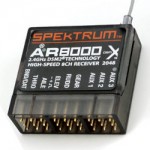
Spektrum DX9 Tx & Spektrum AR8000 Rx

250x250: Spektrum DX9 9-ch RC Tx
Spektrum DX9 9-ch RC Tx

250x250: Spektrum AR8000 Rx
Spektrum AR8000 Rx

Table 1
The Spektrum DX9 Tx & Spektrum AR8000 Rx shows a PWM range from 921 µs to 2129 µs. The following table shows the details of my data capture session:

Spektrum DX9 Tx & Spektrum AR8000 Rx
Tx	Avg PWM	Min	Max	Width	Middle
150	2123.57	2119	2129	10	2124.0
149	2119.40	2113	2124	11	2118.5
148	2115.38	2109	2121	12	2115.0
147	2111.07	2105	2116	11	2110.5
146	2106.94	2101	2111	10	2106.0
100	1923.78	1918	1929	11	1923.5
50	1724.52	1720	1729	9	1724.5
0	1525.23	1520	1531	11	1525.5
-50	1325.74	1319	1331	12	1325.0
-100	1126.63	1122	1132	10	1127.0
-120	1047.06	1041	1051	10	1046.0
-135	987.40	983	992	9	987.5
-146	943.40	939	948	9	943.5
-147	939.48	935	944	9	939.5
-148	935.34	929	940	11	934.5
-149	931.24	926	936	10	931.0
-150	927.43	921	932	11	926.5

Table 2
From these values, I extracted the following polynomial functions:

Polynomial Equation	Py1	Px1	Py2	Px2	a2	a1	a0
0	150	2123.57	-150	927.43	0	0.25080676	-382.605213
1	146	2106.94	-135	987.40	0	0.25099594	-382.8344
2	100	1923.78	-100	1126.63	0	0.25089444	-382.665703
3	148	2115.38	-148	935.34	0	0.25083895	-382.619708
4	146	2106.94	-146	943.40	0	0.25095742	-382.75323
5	149	2119.40	-149	931.24	0	0.25080797	-382.563419
6					-1.0E-07	0.2513	-382.95

Table 3
Again, calculating the performance of each polynomial functions:

Tx	Average PWM	Eq0	Diff 0	Eq1	Diff 1	Eq2	Diff 2	Eq3	Diff 3	Eq4	Diff 4	Eq5	Diff 5	Eq6	Diff 6
150	2123.57	150	0	150	0.17	150	0.13	150	0.05	150	0.17	150	0.04	150	0.25
149	2119.40	149	0.04	149	0.13	149	0.08	149	0.01	149	0.13	149	0	149	0.21
148	2115.38	148	0.05	148	0.12	148	0.07	148	0	148	0.12	148	0.01	148	0.2
147	2111.07	147	0.14	147	0.04	147	0.01	147	0.08	147	0.03	147	0.09	147	0.12
146	2106.94	146	0.17	146	0	146	0.05	146	0.12	146	0	146	0.13	146	0.08
100	1923.78	100	0.11	100	0.03	100	0	100	0.06	100	0.03	100	0.06	100	0.13
50	1724.52	50	0.08	50	0.01	50	0.01	50	0.04	50	0.03	50	0.04	50	0.13
0	1525.23	0	0.07	0	0.01	0	0.01	0	0.03	0	0.02	0	0.02	0	0.11
-50	1325.74	-50	0.1	-50	0.08	-50	0.04	-50	0.07	-50	0.05	-50	0.06	-50	0.03
-100	1126.63	-100	0.04	-100	0.05	-100	0	-100	0.02	-100	0.02	-100	0	-100	0.05
-120	1047.06	-120	0	-120	0.03	-120	0.04	-120	0.02	-120	0.01	-120	0.05	-120	0.07
-135	987.40	-135	0.04	-135	0	-135	0.07	-135	0.06	-135	0.04	-135	0.09	-135	0.09
-146	943.40	-146	0.01	-146	0.04	-146	0.03	-146	0.02	-146	0	-146	0.05	-146	0.04
-147	939.48	-147	0.02	-147	0.03	-147	0.05	-147	0.04	-147	0.02	-147	0.07	-147	0.05
-148	935.34	-148	0.02	-148	0.07	-148	0.01	-148	0	-148	0.02	-148	0.03	-148	0.01
-149	931.24	-149	0.04	-149	0.1	-149	0.02	-149	0.03	-149	0.05	-149	0	-149	0.02
-150	927.43	-150	0	-150	0.05	-150	0.02	-150	0.02	-150	0.01	-150	0.04	-150	0.03
			0.93		0.95		0.62		0.67		0.75		0.78		1.59

The table above shows two polynomial functions (see highlighted columns) that offers the best performance :

Function #2 (which has an order of 1) and a sum of 0.62.
Function #6 (which has an order of 2) and a sum of 1.59.

Function #2 offers the best performance. It is even better than the polynomial function with an order of 3. All control points matches the expected values. This means that Spektrum AR8000 Rx delivers near-perfect and linear PWM values for all given transmitter values.

The following polynomial function offers the best performance to compute the Spektrum DX9 RC Transmitter value from the Spektrum AR8000 Rx pulse length:

f(x) = 0.25089444*x – 382.665703

Download the Spektrum DX9 Tx & Spektrum AR8000 Rx (544 downloads) full data capture.

Tactic TTX600 Tx & Tactic TR624 Rx

250x250: Tactic TTX600 6-ch Tx.jpg
Tactic TTX600 6-ch Tx.jpg

250x250: Tactic TR624 6-ch Rx
Tactic TR624 6-ch Rx

Notes:
The TTX600 transmitter is not digital. This means that it is hard to reproduce the exact behavior every time. As you can see the result are pretty erratic. Each different channel has a different behavior.

For extracting the data, I assumed that moving any sticks to the top, bottom, left and right position would always match a perfect 100% (or -100%). Other values (+60%, -60%) are based on the documentation manual which states that high and low dual rates are based on a 100% and 60% ratio.

Note that each channel section are identified by a unique color which helps to identify the source of each Polynomial Equation.

Table 1
The Tactic TTX600 Tx & Tactic TR624 Rx shows a PWM range from 984 µs to 2030 µs. The following table shows the details of my data capture session:

Tactic TTX600 tx & Tactic TR624
Tx	Avg PWM	Min	Max	Width	Middle	Comment
100	1969.01	1962	1973	11	1967.5	CH1 +100
60	1793.74	1789	1800	11	1794.5	CH1 +60
0	1502.62	1498	1508	10	1503.0	CH1 0
-60	1214.30	1209	1219	10	1214.0	CH1 -60
-100	1042.41	1037	1046	9	1041.5	CH1 -100
100	2022.89	2017	2030	13	2023.5	CH2 +100
60	1838.71	1834	1844	10	1839.0	CH2 +60
0	1530.52	1526	1536	10	1531.0	CH2 0
-60	1230.26	1226	1235	9	1230.5	CH2 -60
-100	1048.09	1043	1052	9	1047.5	CH2 -100
100	2010.15	2004	2016	12	2010.0	CH5 +100
-100	989.31	985	995	10	990.0	CH5 -100
100	2010.39	2004	2016	12	2010.0	CH6 +100
-100	989.40	984	994	10	989.0	CH6 -100

Table 2
From these values, I extracted the following polynomial functions:

Polynomial Equation	Py1	Px1	Py2	Px2	a2	a1	a0
0	100	2010.152	-100	989.308	0	0.19591632	-293.821583
1	100	2010.392	-100	989.402	0	0.1958883	-293.81228
2	100	2022.892	-100	1048.088	0	0.20516945	-315.035638
3	60	1838.708	-60	1230.256	0	0.1972218	-302.633306
4	100	2022.892	-60	1230.256	0	0.2018581	-308.337143
5	60	1838.708	-100	1048.088	0	0.20237282	-312.104526
6	all control points				9.00E-06	0.1755	-287.34
7	CH1 control points				-3.00E-06	0.2221	-327.22
8	CH2 control points				-3.00E-06	0.2135	-318.97

Table 3 (for CH1)
The following table shows details for calculating the performance of each polynomial functions:

Tx	Avg PWM	Eq2	Diff 2	Eq3	Diff 3	Eq4	Diff 4	Eq5	Diff 5	Eq6	Diff 6	Eq7	Diff 7	Eq8	Diff 8
100	1969.01	89	11.05	86	14.3	89	10.88	86	13.63	93	6.89	98	1.53	90	10.22
60	1793.74	53	7.02	51	8.87	54	6.26	51	9.1	56	3.58	62	1.52	54	5.66
0	1502.62	-7	6.74	-6	6.28	-5	5.02	-8	8.02	-3	3.31	0	0.26	-5	4.93
-60	1214.30	-66	5.9	-63	3.15	-63	3.22	-66	6.36	-61	0.96	-62	1.95	-64	4.14
-100	1042.41	-101	1.17	-97	2.95	-98	2.08	-101	1.15	-95	5.38	-99	1.04	-100	0.32
			31.88		35.55		27.46		38.26		20.12		6.3		25.28

Table 3 (for CH2)
The following table shows details for calculating the performance of each polynomial functions:

Tx	Avg PWM	Eq2	Diff 2	Eq3	Diff 3	Eq4	Diff 4	Eq5	Diff 5	Eq6	Diff 6	Eq7	Diff 7	Eq8	Diff 8
100	2022.89	100	0	96	3.67	100	0	97	2.73	105	4.51	110	9.79	101	0.64
60	1838.71	62	2.21	60	0	63	2.82	60	0	66	5.78	71	11.01	63	3.45
0	1530.52	-1	1.02	-1	0.78	1	0.61	-2	2.37	2	2.35	6	5.68	1	0.77
-60	1230.26	-63	2.62	-60	0	-60	0	-63	3.13	-58	2.19	-59	1.48	-61	0.85
-100	1048.09	-100	0	-96	4.07	-97	3.23	-100	0	-94	6.49	-98	2.26	-98	1.5
			5.85		8.53		6.66		8.23		21.31		30.23		7.21

The two tables above shows two polynomial functions (see highlighted columns) that offers the best performance:

Function #7 (which has an order of 2) and a sum of 6.3.
Function #8 (which has an order of 2) and a sum of 7.21.
All polynomial function which has an order of 1 shows terrible prediction performance.

Note that best function for channel 1 (function #7) shows terrible results when used in calculations of channel 2. That is also for function 8. This means that there is no generic function that can be used for all channel situations. As a proof, function #6 which is based on all observed values for all channels shows terrible results.

In other words, reading the PWM length or the Tactic TTX600 Tx & Tactic TR624 Rx combination can only be used for detecting if the sticks are “up”, “centered” or “down” but not really “how much up or down”.

The following polynomial functions offers the best performance to compute the Tactic TTX600 Tx transmitter value from the Tactic TR624 Rx pulse length:

Channel 1 :

f(x) = -3.0E-6*x² + 0.2221*x – 327.22

Channel 2 :

f(x) = -3.0E-6*x2 + 0.2135*x – 318.97

Download the Tactic TTX600 Tx & Tactic TR624 Rx (560 downloads) full data capture.

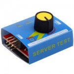
CCPM Servo Tester

250x250: CCPM Servo Tester
CCPM Servo Tester

Table 1
The CCPM Servo Tester shows a PWM range from 900 µs to 2210 µs. The following table shows the details of my data capture session:

CCPM Servo Tester
Value	Avg PWM	Min	Max	Width	Middle	Comment
100	2103.82	2098	2110	12	2104	CW
0	1504.75	1501	1511	10	1506	CENTER
-100	903.77	900	909	9	904.5	CCW

Note that values for the CCPM Server Tester (100, -100) are assumptions and represents clockwise and counterclockwise positions of the potentiometer. In fact, based on the observed PWM values, the values should be more in the (133, -133) range according the Spektrum DX9 Tx & Orange R620X Rx results or in (150, -150) range according the Spektrum DX9 Tx & Spektrum AR8000 Rx results.

Table 2
From these values, I extracted the following polynomial functions:

Polynomial Equation	Py1	Px1	Py2	Px2	a2	a1	a0
0	100	2103.82	-100	903.77	0	0.16665945	-250.62214
1	100	2103.824	0	1504.752	0	0.16692484	-251.180493
2	0	1504.752	-100	903.772	0	0.16639489	-250.383041
3					4.0E-07	0.1653	-249.78

Table 3
The following table shows details for calculating the performance of each polynomial functions:

Value	Avg PWM	Eq0	Diff 0	Eq1	Diff 1	Eq2	Diff 2	Eq3	Diff 3
100	2103.82	100	0	100	0	100	0.32	100	0.25
0	1504.75	0	0.16	0	0	0	0	0	0.14
-100	903.77	-100	0	-100	0.32	-100	0	-100	0.06
			0.16		0.32		0.32		0.45

Note that only 3 control points are available which means that all performance calculations will always match 2/3 controls points (since the equation is derived from these 2 points). Performance calculations are irrelevant in this particular situation.

Even if the performance of function #3 seem to be the worst, it seems like it is the one that is the most promising since it takes into account all control points.

The following polynomial function offers the best performance to compute the CCPM Servo Tester pulse length:

f(x) = 4.0E-07*x² + 0.1653*x – 249.78

Download the CCPM Servo Tester (560 downloads) full data capture.

end2end zone

Mapping RC Transmitter PWM signal to actual transmitter values

Introduction

How does it works?

What is expected

Theoretical values

Extrapolation

Capture methodology

Required Libraries

PinChangeInt

eRCaGuy_Timer2_Counter

PWM capture code

Benchmark results

Devices

Spektrum DX9 Tx & Orange R620X Rx

Spektrum DX9 Tx & Spektrum AR8000 Rx

Tactic TTX600 Tx & Tactic TR624 Rx

CCPM Servo Tester

Leave a Reply Cancel reply

My life dumped to a web site